When failure occurs in Ceph, or when more OSDs are added to a cluster, data moves around to re-replicate objects or to re-balance data placement. This movement is minimized by design, but sometimes it is necessary to scale the system in a way that causes a lot of data movement, and will have an impact on performance (though in practice this is a rare event for which scheduled downtime may be reasonable). This post examines very briefly the performance impact in a constrained set of microbenchmarks.
An object in RADOS maps to a placement group, and each placement group maps to
one or more physical devices. The essence of the first mapping is captured by
the function pg = hash(oid) % pg_num which given an object name oid
selects a target placement group from the range 0..pg_num. The second
mapping is more complex, based on CRUSH, but computes something analogous to
osd = hash(pg) % pgp_num where pgp_num is the number of placement group
placements, or something like the number of OSDs being considered for
placement (I think this definition may not be very precise). The important
thing is that when OSDs are added, a minimum number of placement groups are
moved (and by extension a minimum number of objects).
A typical Ceph deployment will choose a large number of placement groups, on the order of 100s per OSD, so when new hardware is added some placement groups can be re-mapped for balancing, but it is proportional to the expansion of the cluster. When the ratio of PGs to OSDs becomes small adding new placement groups may be required. In affect the addition of placement groups changes the mapping between objects and placement groups, and can incur significant data movement as PGs are effectively being split. In this post we are interested in what the effect of this splitting is on client operation latency.
We’ll start with a microbenchmark that consists of a single client calling
rados::create() on objects named obj.0,1,2,.... The client generates this
workload on a pool with a single placement group. After some period of time we
add an additional placement group to the pool and observe changes in latency
as the system adjusts. The experiments are run on a beefy system with 384 GB
RAM and 16 cores. On this system 2 OSDs are deployed and backed by the
in-memory object store. The purpose of using the in-memory store is to remove
as much noise as possible (sources of which include network and storage
devices) to expose the system behavior.
Results
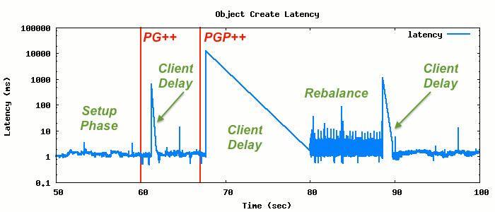
The annotated graph below shows the phases of the experiment. The setup
phase consists of the client running without any changes to the system.
During this phase the single placement group in the pool is being populated
with objects (of zero length). In the example here we perform this setup for
sixty seconds (note that we clip the graph up to this point). The next phase
starts when we instruct Ceph to add an additional placement group (labeled
PG++). Notice a small interruption to client performance immediately
following this. Once the system stabilizes we increase the number of PG
placements. Following this is a longer client delay followed by a period of
increased latency, presumably while Ceph is rebalancing. This period is
followed by a final, short delay.
Each experiment follows the same basic structure but we increase the amount of time before we split the placement group. The reasoning behind this is that we would like to know how latency is affected by the size of the placement group at the time we perform the split. In the following experiment we double the setup time to two minutes. Note that this corresponds to approximately 95,000 objects, in contrast to the previous example that had a 60 second setup time corresponding to around 47,000 objects.
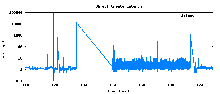
In the second example, although we have doubled the start-up time, the time in the rebalance phase is approximately three times as long at 30 seconds, but note that the client delay immediately preceding the rebalance is approximately 10 seconds in each case. In the next experiment we increase the setup time again to 300 seconds, or approximately 250,000 objects.
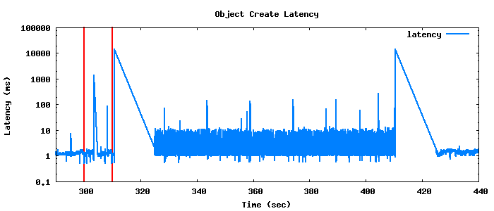
And we can keep doing this all day, but I’ll just summarize the results in this nice table, as these graphs quickly become very crowded by the rebalance phase and obscure the other phases.
| phase/setup-time | 120s | 300s | 600s | 1200s |
|---|---|---|---|---|
| num objs | 95K | 250K | 512K | 975K |
| pg delay | 1s | 1s | 2s | 4s |
| pgp delay | 12s | 14s | 11s | 12s |
| shuffle | 27s | 86s | 195s | 380s |
| post shuffle delay | 1s | 16s | 1s | 1s |
Next Steps
The next thing we’ll be looking at are other operations such as reading and writing during PG splitting. We’ll focus first on these microbenchmarks and then start to expand into full scale benchmarks. It’d also be interesting to look at the performance of concurrent workloads because operations will be unblocked as data is fully migrated, and this is an iterative process that takes time.